Welcome to statTarget !
Quality Control (QC) has been considered as an essential step in the
MS-based omics platform for high reproducibility and accuracy of data.
The repetitive use of the same QC samples is more and more accepted for
evaluation and correction of the signal drift during the sequence of MS run order,
especially beneficial to improve the quality of data in multi-blocks
experiments (Dunn, W.B., et al., 2011). statTarget is a streamlined tool
to provide a graphical user interface for quality control based
signal correction, and integration of MS data from multi-batch of
experiments, and comprehensive statistic analysis for
MS-based Omics data.
This document is intended to guide the user to use the functions to
perform data analysis, such as shiftCor, statAnalysis, statTargetGUI functions, etc.

Package overview
A streamlined tool provides graphical user interface for quality control based signal correction, integration of metabolomics and proteomics data from multi-batch experiments, and the comprehensive statistic analysis.
(URL: https://stattarget.github.io)
Citation
Please cite the following article when using statTarget or QC-RFSC algorithm:
Luan H., Ji F., Chen Y., Cai Z. (2018) statTarget: A streamlined tool for signal drift correction and interpretations of quantitative mass spectrometry-based omics data. Analytica Chimica Acta. dio: https://doi.org/10.1016/j.aca.2018.08.002
Luan H., Ji F., Chen Y., Cai Z. (2018) Quality control-based signal drift correction and interpretations of metabolomics/proteomics data using random forest regression. bioRxiv 253583; doi: https://doi.org/10.1101/253583
What does statTarget offer statistically
The statTarget has two basic sections. The first section
is Signal Correction (See the shiftCor function). It includes ‘Ensemble Learning’ for QC based signal correction. For example, QC-based random forest correction (QC-RFSC) and QC-based LOESS signal correction (QCRLSC). (Dunn WB., et al. 2011; Luan H., et al. 2015). The second
section is Statistical Analysis (See the statAnalysis function). It provides comprehensively computational and statistical methods that are commonly applied to analyze Omics data,
and offers multiple results for biomarker discovery. The statTargetGUI provides the simple easy to use interface for the above functions.
Section 1 - Signal Correction provide ensemble learning method for QC based signal correction. i.e. QC based random forest signal correction (QC-RFSC) that fit the QC data,
and each metabolites in the true sample will be normalized to the QC sample.
Section 2 - Statistical Analysis provide features including Data preprocessing, Data descriptions, Multivariate statistics analysis and Univariate analysis.
Data preprocessing : 80-precent rule, sum normalization (SUM) and probabilistic quotient normalization (PQN), glog transformation, KNN imputation, median imputation, and minimum imputation.
Data descriptions : Mean value, Median value, sum, Quartile, Standard
derivatives, etc.
Multivariate statistics analysis : PCA, PLSDA, VIP, Random forest, Permutation-based feature selection.
Univariate analysis : Welch’s T-test, Shapiro-Wilk normality test and Mann-Whitney test.
Biomarkers analysis: ROC, Odd ratio, Adjusted P-value, Box plot and Volcano plot.
statTargetGUI
## Examples Code for graphical user interface

library(statTarget)

statTargetGUI()

#For mac PC,  the GUI function 'statTargetGUI()' need the XQuartz instead of X11 support. Download it from https://www.xquartz.org. R 3.3.0 and RGtk2 2.20.31 are recommended for RGtk2 installation.

statTargetGUI
Download the Reference manual and example data .
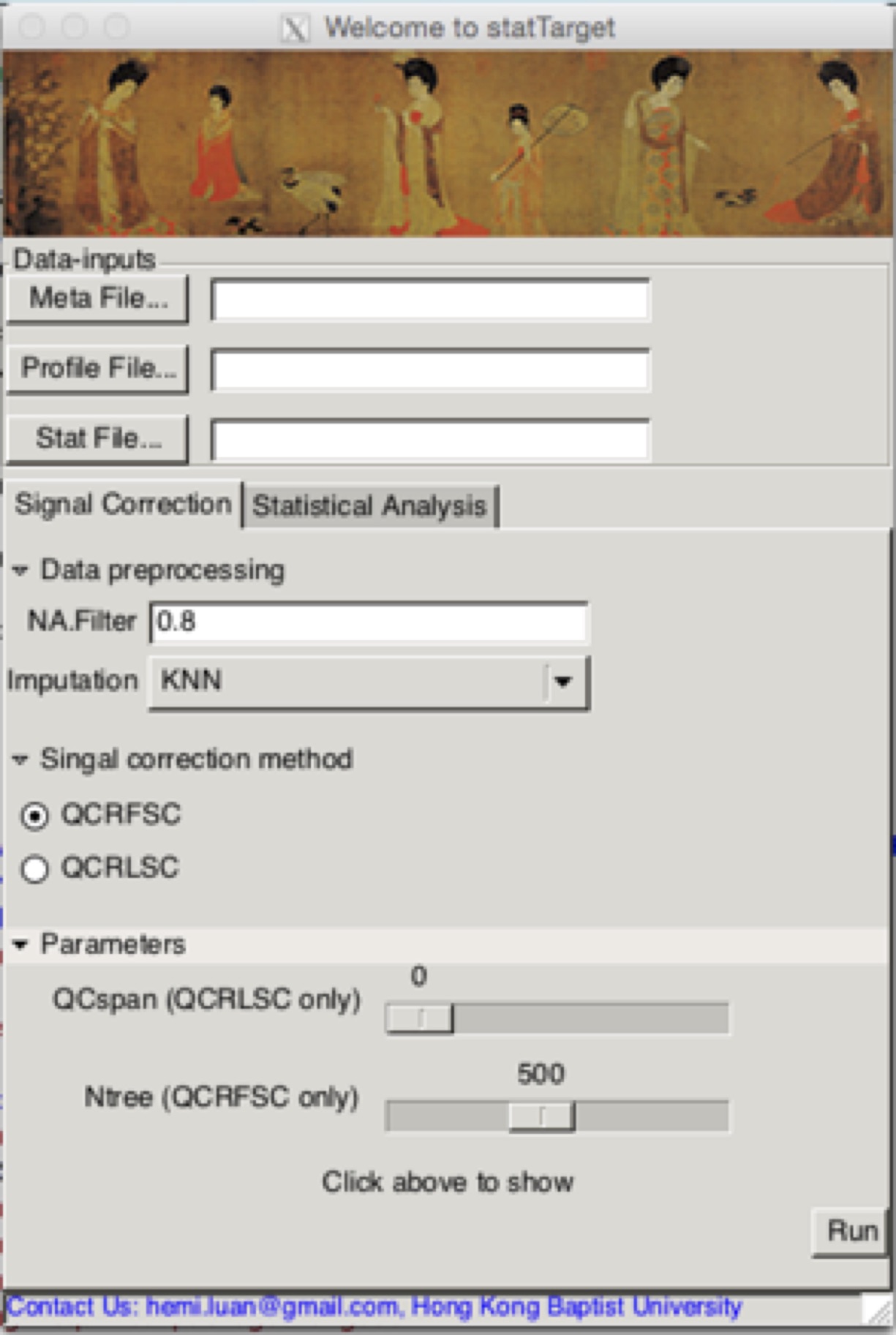
Running Signal Correction (the shiftCor function) from the GUI
Meta File
Meta information includes the Sample name, class, batch and order.
Do not change the name of each column
(1) Class: The QC should be labeled as NA
(2) Order : Injection sequence.
(3) Batch: The analysis blocks or batches
(4) Sample name should be consistent in Meta file and Profile file
(See the example data)
Profile File
Expression data includes the sample name and expression
data.(See the example data)
NA.Filter
Modified n precent rule function. A variable will be kept if it has a non-zero value for at least n precent of samples in any one group. (Default: 0.8)
MLmethod
The machine learning method for QC based signal correction. i.e. QC-RFSC, QC-RLSC.
Ntree
Number of trees to grow for QC-RFSC (Default: 500) .
QCspan
The smoothing parameter for QCRLSC which controls the bias-variance tradeoff.
The common range of QCspan value is from 0.5 to 0.75. If you choose
a span that is too small then there will be a large variance.
If the span is too large, a large bias will be produced.
The default value of QCspan is set at ‘0’, the generalised
cross-validation will be performed for choosing a good value,
avoiding overfitting of the observed data. (Default: 0)
Imputation
The parameter for imputation method.(i.e.,
nearest neighbor averaging, “KNN”; minimum values, “min”; Half of minimum values
“minHalf” median values, “median”. (Default: KNN)
## Examples Code

library(statTarget)

datpath <- system.file('extdata',package = 'statTarget')
samPeno <- paste(datpath,'MTBLS79_sampleList.csv', sep='/')
samFile <- paste(datpath,'MTBLS79.csv', sep='/')
shiftCor(samPeno,samFile, Frule = 0.8, MLmethod = "QCRFSC", QCspan = 0,imputeM = "KNN")

See ?shiftCor for off-line help
Running Statistical Analysis (the statAnalysis function) from the GUI
Stat File
Expression data includes the sample name, group, and expression data.
NA.Filter
Modified n precent rule function. A variable will be kept if it has a non-zero value for at least n precent of samples in any one group. (Default: 0.8)
Imputation
The parameter for imputation method.(i.e., nearest neighbor averaging, “KNN”;
minimum values, “min”; Half of minimum values “minHalf”; median values,
“median”. (Default: KNN)
Normalization
The parameter for normalization method (i.e probabilistic quotient
normalization, “PQN”; integral normalization , “SUM”, and “none”).
Glog
Generalised logarithm (glog) transformation for Variance stabilization
(Default: TRUE)
Scaling Method
Scaling method before statistic analysis i.e. PCA or PLS(DA).
Center can be used for specifying the Center scaling.
Pareto can be used for specifying the Pareto scaling.
Auto can be used for specifying the Auto scaling (or unit variance scaling).
Vast can be used for specifying the vast scaling.
Range can be used for specifying the Range scaling. (Default: Pareto)
Permutation times
The number of permutation times for cross-validation of PLS-DA model, and variable importance of randomforest model
PCs
PCs in the Xaxis or Yaxis: Principal components in
PCA-PLS model for the x or y-axis (Default: 1 and 2)
nvarRF
The number of variables with top permutation importance in randomforest model.
(Default: 20)
Labels
To show the name of sample or groups in the Score plot. (Default: TRUE)
Multiple testing
This multiple testing correction via false discovery rate (FDR)
estimation with Benjamini-Hochberg method. The false discovery rate
for conceptualizing the rate of type I errors in null hypothesis
testing when conducting multiple comparisons. (Default: TRUE)
Volcano FC
The up or down -regulated metabolites using Fold Changes cut off
values in the Volcano plot. (Default: > 2 or < 0.5)
Volcano Pvalue
The significance level for metabolites in the Volcano plot.(Default: 0.05)
## Examples Code

library(statTarget)

datpath <- system.file('extdata',package = 'statTarget')
file <- paste(datpath,'data_example.csv', sep='/')
statAnalysis(file,Frule = 0.8, normM = "NONE", imputeM = "KNN", glog = TRUE,scaling = "Pareto")
The transX function is to generate statTarget input file formats from Mass Spectrometry Data softwares, such as XCMS, MZmine2, SIEVE and SKYLINE. ‘?transX’ for off-line help.
## Examples Code

library(statTarget)

datpath <- system.file('extdata',package = 'statTarget')
dataXcms <- paste(datpath,'xcmsOutput.tsv', sep='/')
dataSkyline <- paste(datpath,'skylineDemo.csv', sep='/')
transX(dataXcms,'xcms')
transX(dataSkyline,'skyline')

See ?transX for off-line help
Random Forest classfication and variable importance measures
rForest provides the Breiman’s random forest algorithm for classification and permutation-based variable importance measures (PIMP-algorithm).
## Examples Code

library(statTarget)

datpath <- system.file('extdata',package = 'statTarget')
statFile <- paste(datpath,'data_example.csv', sep='/')
getFile <- read.csv(statFile,header=TRUE)

# Random Forest classfication
rFtest <- rForest(getFile,ntree = 10,times = 5)

# Prediction of test data using random forest in statTarget.
predictOutput <- predict_RF(rFtest, getFile[1:19,3:8])

# Multi-dimensional scaling plot of proximity matrix from randomForest.
mdsPlot(rFtest$randomForest,rFtest$pimpTest)

# Create plots for Gini importance and permutation-based variable Gini importance measures.
pvimPlot(rFtest$randomForest,rFtest$pimpTest)

graphics.off()

See ?rForest for off-line help
Investigation of the results
Download the Example data and Demo reports
Once data files have been analysed it is time to investigate them.
Please get this info. through the GitHub page.
(URL: https://stattarget.github.io)
Results of Signal Correction (ShiftCor)
statTarget -- shiftCor
-- After_shiftCor             # The fold for intergrated and corrected data
   -- shift_all_cor.csv         # The corrected data of samples and QCs
   -- shift_QC_cor.csv          # The corrected data of QCs only
   -- shift_sample_cor.csv      # The corrected data of samples only
   -- loplot                    # The fold for quality control images
      -- *.pdf                  # The quality control images for each features

-- Before_shiftCor            # The fold for raw data
   -- shift_QC_raw.csv          # The raw data of QCs
   -- shift_sam_raw.csv         # The raw data of samples

-- RSDresult                  # The fold for variation analysis and quality assessment
   -- RSD_all.csv               # The RSD values of each feature
   -- RSDdist_QC_stat.csv       # The RSD distribution of QCs in each batch and all batches
   -- RSD distribution.pdf      # The RSD distribution plot in samples and QCs of all batches
   -- RSD variation.pdf         # The RSD variation plot for pre- and post- signal correction
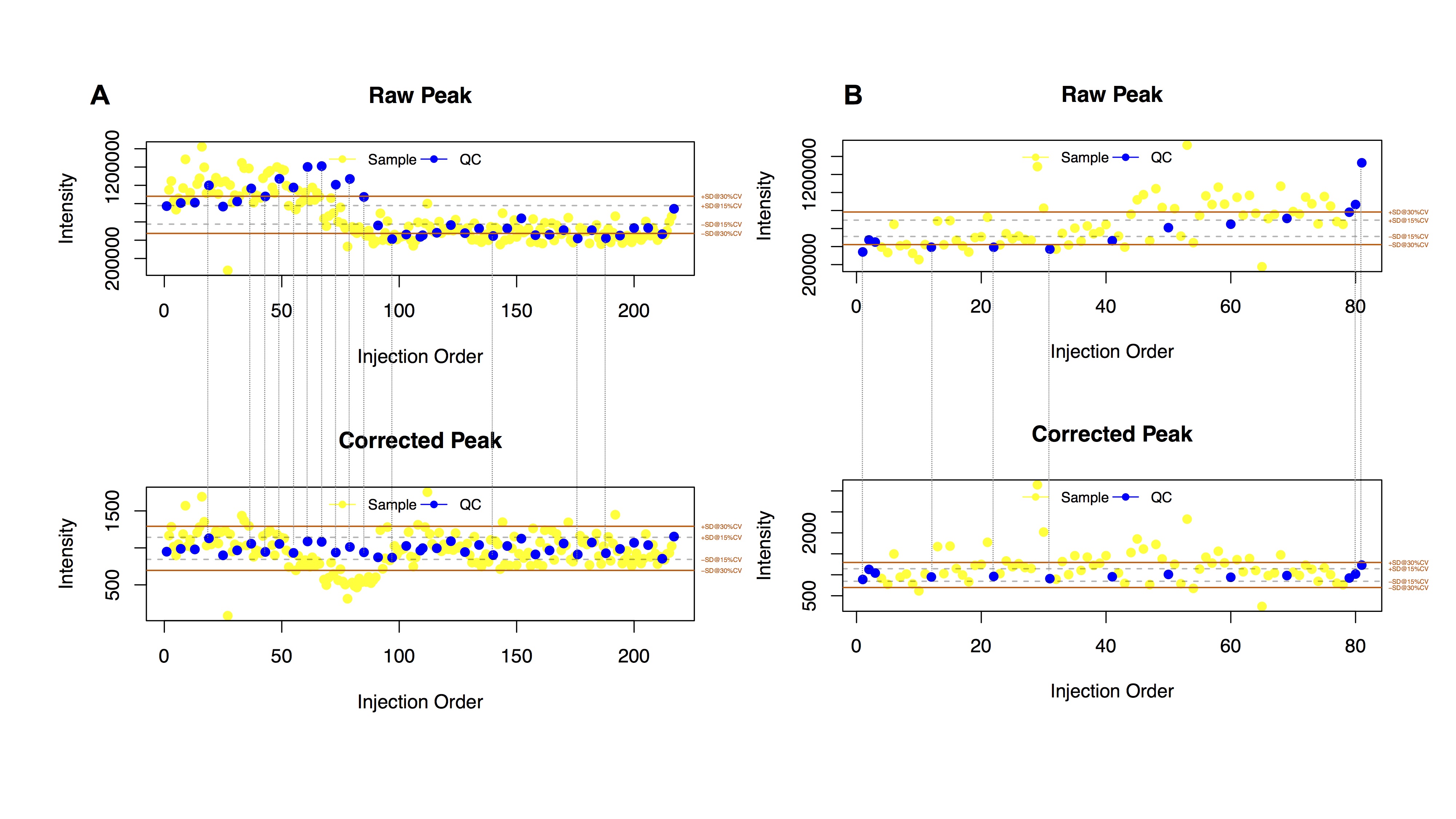
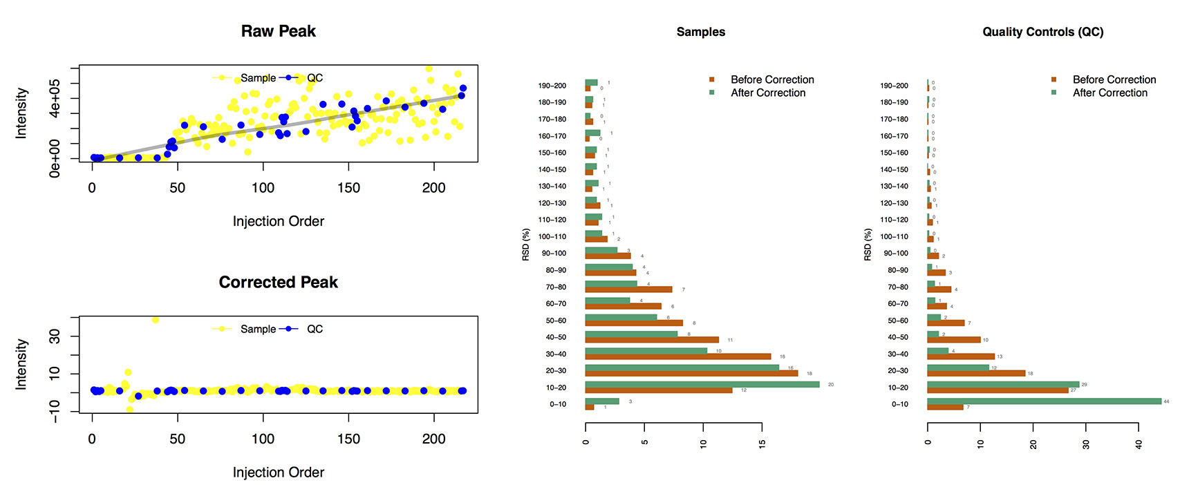
Loplot (left): the visible image of quality control images for each features
The RSD distribution (right):
The relative standard deviation of peaks in the samples and QCs

- The status log (Example data):
#############################
# Signal Correction function #
#############################


statTarget: Shift Correction Start... Time: Sun Mar 19 19:43:25 2017

* Step 1: Data File Checking Start..., Time:  Sun Mar 19 19:43:25 2017

 217 Meta Samples vs 218 Profile samples
 The Meta samples list (*NA, missing data from the Profile File)

  [1] "QC1"              "A1"               "A2"               "A3"
  [5] "A4"               "A5"               "QC2"              "A6"
  [9] "A7"               "A8"               "A9"               "A10"
 [13] "QC3"              "A11"              "A12"              "A13"
 [17] "A14"              "A15"              "QC4"              "B16"
 [21] "B17"              "B18"              "B19"              "B20"
 [25] "QC5"              "B21"              "B22"              "B23"
 [29] "B24"              "B25"              "QC6"              "B26"
 [33] "B27"              "B28"              "B29"              "B30"
 [37] "QC7"              "C31"              "C32"              "C33"
 [41] "C34"              "C35"              "QC8"              "C36_120918171155"
 [45] "C37"              "C38"              "C39"              "C40"
 [49] "QC9"              "C41"              "C42"              "C43"
 [53] "C44"              "C45"              "QC10"             "D46"
 [57] "D47"              "D48"              "D49"              "D50"
 [61] "QC11"             "D51"              "D52"              "D53"
 [65] "D54"              "D55"              "QC12"             "D56"
 [69] "D57"              "D58"              "D59"              "D60"
 [73] "QC13"             "E61"              "E62"              "E63"
 [77] "E64"              "E65"              "QC14"             "E66"
 [81] "E67"              "E68"              "E69"              "E70"
 [85] "QC15"             "E71"              "E72"              "E73"
 [89] "E74"              "E75"              "QC16"             "F76"
 [93] "F77"              "F78"              "F79"              "F80"
 [97] "QC17"             "F81"              "F82"              "F83"
[101] "F84"              "F85"              "QC18"             "F86"
[105] "F87"              "F88"              "F89"              "F90"
[109] "QC19"             "QC20"             "a1"               "a2"
[113] "a3"               "a4"               "a5"               "QC21"
[117] "a6"               "a7"               "a8"               "a9"
[121] "a10"              "QC22"             "a11"              "a12"
[125] "a13"              "a14"              "a15"              "QC23"
[129] "b16"              "b18"              "b19"              "b20"
[133] "b21"              "QC24"             "b22"              "b23"
[137] "b24"              "b25"              "b26"              "QC25"
[141] "b27"              "b28"              "b29"              "b30"
[145] "c31"              "QC26"             "c32"              "c33"
[149] "c34"              "c35"              "c36"              "QC27"
[153] "c37"              "c38"              "c39"              "c40"
[157] "c41"              "QC28"             "c42"              "c43"
[161] "c44"              "c45"              "d46"              "QC29"
[165] "d47"              "d48"              "d49"              "d50"
[169] "d51"              "QC30"             "d52"              "d53"
[173] "d54"              "d55"              "d56"              "QC31"
[177] "d57"              "d58"              "d59"              "d60"
[181] "e61"              "QC32"             "e62"              "e63"
[185] "e64"              "e65"              "e66"              "QC33"
[189] "e67"              "e68"              "e69"              "e70"
[193] "e71"              "QC34"             "e72"              "e73"
[197] "e74"              "e75"              "f76"              "QC35"
[201] "f77"              "f78"              "f79"              "f80"
[205] "f81"              "QC36"             "f82"              "f83"
[209] "f84"              "f85"              "f86"              "QC37"
[213] "f87"              "f88"              "f89_120921102721" "f90"
[217] "QC38"

 Warning: The sample size in Profile File is larger than Meta File!

 Meta-information:

  Class No.
1     1  30
2     2  29
3     3  30
4     4  30
5     5  30
6     6  30
7    QC  38
  Batch No.
1     1 109
2     2 108

 Metabolic profile information:

                no.
QC and samples  218
Metabolites    1312

* Step 2: Evaluation of Missing Value...

 The number of missing value before QC based shift correction:  2280
 The number of variables including 80 % of missing value :   3

* Step 3: Imputation start...

 The imputation method was set at 'KNN'
 The number of missing value after imputation:  0
 Imputation Finished!

* Step 4: QC-based Shift Correction Start... Time:  Sun Mar 19 19:43:28 2017

 The MLmethod was set at QCRFC

  |
  |                                                                          |   0%
  |
  |=                                                                         |   1%
  |
  |=                                                                         |   2%
  |
  |==                                                                        |   2%
  |
  |==                                                                        |   3%
   ...
  |========================================================================  |  98%
  |
  |========================================================================= |  99%
  |
  |==========================================================================|  99%
  |
  |==========================================================================| 100%

 High-resolution images output...

  |
  |                                                                          |   0%
  |
  |                                                                          |   1%
  |
  ...
  |========================================================================  |  98%
  |
  |========================================================================= |  99%
  |
  |==========================================================================|  99%
  |
  |==========================================================================| 100%

 Calculation of CV distribution of raw peaks (QC)...

            CV<5%    CV<10%   CV<15%   CV<20%   CV<25%   CV<30%   CV<35%   CV<40%
Batch_1 0.4583652  7.868602 22.84186 36.74561 46.37128 53.32315 60.80978 66.99771
Batch_2 6.5699007 29.870130 49.50344 59.12911 65.62261 70.58824 76.01222 80.67227
Total   0.3819710  6.875477 21.31398 33.68984 44.61421 52.10084 59.12911 65.01146
          CV<45%   CV<50%   CV<55%   CV<60%   CV<65%   CV<70%   CV<75%   CV<80%
Batch_1 72.49809 77.76929 81.05424 84.03361 86.93659 88.54087 89.53400 90.60351
Batch_2 83.34607 86.78380 89.22842 90.98549 92.20779 93.35371 94.27044 94.95798
Total   69.44232 74.17876 78.38044 81.20703 83.11688 85.10313 87.01299 89.99236
          CV<85%   CV<90%   CV<95%  CV<100%
Batch_1 91.59664 92.74255 93.65928 94.88159
Batch_2 95.79832 96.40947 96.71505 97.32620
Total   91.74943 93.43010 94.57601 95.03438

 Calculation of CV distribution of corrected peaks (QC)...

           CV<5%   CV<10%   CV<15%   CV<20%   CV<25%   CV<30%   CV<35%   CV<40%
Batch_1 20.77922 53.93430 70.20626 80.21390 85.71429 89.61039 92.13140 93.58289
Batch_2 33.61345 63.02521 78.38044 86.70741 91.06188 93.88846 94.80519 95.87471
Total   22.76547 54.92743 73.79679 83.11688 88.15890 90.90909 93.04813 94.27044
          CV<45%   CV<50%   CV<55%   CV<60%   CV<65%   CV<70%   CV<75%   CV<80%
Batch_1 94.42322 95.18717 95.79832 96.25668 97.32620 97.86096 98.39572 98.62490
Batch_2 96.25668 97.17341 97.78457 98.16654 98.47212 98.54851 98.54851 98.77769
Total   95.87471 97.02063 97.78457 98.01375 98.39572 98.54851 98.54851 98.62490
          CV<85%   CV<90%   CV<95%  CV<100%
Batch_1 98.85409 98.93048 98.93048 99.23606
Batch_2 99.00688 99.15966 99.15966 99.15966
Total   98.85409 99.00688 99.23606 99.38885

 Correction Finished! Time:  Sun Mar 19 19:44:54 2017
Results of statistic analysis (statAnalysis)
statTarget -- statAnalysis

-- dataSummary                  # The results summaries of basic statistics
-- scaleData_XX                 # The results of scaling procedure
-- DataPretreatment             # Data processed with normalizationor glog transformation procedure.
-- randomForest                 # The results of randomForest analysis and permutation based importance variables.
   -- MultiDimensionalScalingPlot # Multi dimensional scaling plot
   -- VarableImportancePlot       # Varable importance plot

-- PCA_Data_XX                  # Principal Component Analysis with XX scaling
   -- ScorePlot_PC1vsPC2.pdf      # Score plot for 1st component vs 2st component in PCA analysis
   -- LoadingPlot_PC1vsPC2.pdf    # Loading plot for 1st component vs 2st component in PCA analysis

-- PLS_(DA)_XX                  # Partial least squares (-Discriminant Analysis) with XX scaling
   -- ScorePlot_PLS_DA_Pareto     # Score plot for PLS analysis
   -- W.cPlot_PLS_DA_Pareto       # Loading plot for PLS analysis
   -- Permutation_Pareto          # Permutation test plot for PLS-DA analysis (for two groups only)
   -- PLS_DA_SPlot_Pareto         # Splot plot for PLS analysis

-- Univariate
   ----- BoxPlot
   ----- Fold_Changes             # A ratio of feature between control and case
   ----- Mann-Whitney_Tests       # For non-normally distributed variables
   ----- oddratio                 # Odd ratio
   ----- Pvalues                  # Integration of pvalues or BH-adjusted pvalues for normal data (Welch test) and abnormal data (Mann Whitney Tests)
   ----- ROC                      # Receiver operating characteristic curve
   ----- Shapiro_Tests            # Normality tests
   ----- Significant_Variables    # The features with P-value < 0.05
   ----- Volcano_Plots            # P-value and fold Change scatter plot
   ----- WelchTest                # For normally distributed variables

- The status log (Example data):
#################################
# Statistical Analysis function #
#################################


statTarget: statistical analysis start... Time:  Tue May  9 19:50:53 2017

* Step 1: Evaluation of missing value...

 The number of missing value in Data Profile:  0
 The number of variables including 80 % of missing value :   0

* Step 2: Summary statistics start... Time:  Tue May  9 19:50:53 2017

* Step 3: Missing value imputation start... Time:  Tue May  9 19:50:53 2017

 Imputation method was set at KNN
 The number of NA value after imputation: 0
 Imputation Finished!
* Step 4: Normalization start... Time:  Tue May  9 19:50:59 2017

 Normalization method was set at NONE

* Step 5: Glog PCA-PLSDA start... Time:  Tue May  9 19:51:01 2017

 Scaling method was set at Center

 PCA Model Summary
 59 samples x 1309 variables
 Variance Explained of PCA Model:

                            PC1      PC2      PC3      PC4     PC5
Standard deviation     4.651009 4.452616 3.963728 3.180499 2.66858
Proportion of Variance 0.143390 0.131420 0.104140 0.067050 0.04720
Cumulative Proportion  0.143390 0.274810 0.378950 0.446000 0.49320

 The following observations are calculated as outliers: [1] "A13" "A14"

 PLS(-DA) Two Component Model Summary
 59 samples x 1309 variables
 Fit method: oscorespls
 Number of components considered: 2
 Cross-validated using 10 random segments.

 Cumulative Proportion of Variance Explained: R2X(cum) = 19.34905%
 Cumulative Proportion of Response(s):

                Y1        Y2
R2Y(cum) 0.9391357 0.9391357
Q2Y(cum) 0.8175050 0.8175050

 Permutation of PLSDA Model START...!

  |
  |                                                                               |   0%
  ...
  |===============================================================================|  99%
  |
  |===============================================================================| 100%

* Step 6: Glog Random Forest start... Time:  Tue May  9 19:52:03 2017


  |
  |                                                                               |   0%
  |
  ...
  |============================================================================== |  98%
  |
  |============================================================================== |  99%
  |
  |===============================================================================|  99%
  |
  |===============================================================================| 100%

 Random Forest Model
 Type:  classification
 ntree: 500
 mtry:  36
 OOB estimate of error rate: 0 %

 Permutation-based Gini importance measures
 The number of permutations:  500
 Selected 50 variables with top importance

          1          2          3          4          5          6          7
giniImp   "M302T751" "M301T716" "M304T768" "M113T110" "M279T716" "M305T103" "M117T584"
pvalueImp "M301T716" "M302T751" "M113T110" "M239T109" "M304T768" "M280T750" "M279T716"
          8          9          10         11         12         13         14
giniImp   "M280T750" "M239T109" "M265T768" "M311T103" "M379T103" "M243T104" "M281T750"
pvalueImp "M191T105" "M302T716" "M265T768" "M305T103" "M281T750" "M243T104" "M117T584"
          15         16         17         18         19         20         21
giniImp   "M191T105" "M457T107" "M249T108" "M315T110" "M267T106" "M302T716" "M161T728"
pvalueImp "M311T103" "M379T103" "M249T108" "M283T767" "M267T106" "M305T768" "M315T110"
          22         23         24         25         26         27         28
giniImp   "M283T767" "M305T768" "M348T761" "M297T705" "M355T120" "M259T104" "M263T750"
pvalueImp "M348T761" "M355T120" "M457T107" "M297T705" "M353T761" "M243T754" "M263T750"
          29         30         31         32         33         34         35
giniImp   "M88T588"  "M325T774" "M290T728" "M353T761" "M373T102" "M243T754" "M241T109"
pvalueImp "M241T109" "M107T105" "M259T104" "M325T774" "M290T728" "M161T728" "M262T112"
          36         37         38         39         40           41         42
giniImp   "M338T716" "M262T112" "M107T105" "M381T802" "M165T109_1" "M361T748" "M295T728"
pvalueImp "M381T802" "M338T716" "M88T588"  "M373T102" "M165T109_1" "M261T113" "M295T728"
          43         44         45         46         47         48         49
giniImp   "M239T116" "M261T113" "M205T716" "M761T800" "M269T771" "M283T112" "M257T762"
pvalueImp "M361T748" "M239T116" "M263T115" "M360T748" "M123T105" "M175T104" "M269T771"
          50
giniImp   "M123T105"
pvalueImp "M257T762"

* Step 7: Univariate Test Start...! Time:  Tue May  9 20:01:26 2017

 P-value Calculating...
 P-value was adjusted using Benjamini-Hochberg Method

 Odd.Ratio Calculating...

 ROC Calculating...

  |
  |                                                                               |   0%
  |
  |                                                                               |   1%
  |
  |=============================================================================  |  98%
  |
  |============================================================================== |  98%
  |
  |============================================================================== |  99%
  |
  |===============================================================================|  99%
  |
  |===============================================================================| 100%

 Volcano Plot and Box Plot Output...

 Statistical Analysis Finished! Time:  Tue May  9 20:03:50 2017
References
Dunn, W.B., et al.,Procedures for large-scale metabolic profiling of
serum and plasma using gas chromatography and liquid chromatography coupled
to mass spectrometry. Nature Protocols 2011, 6, 1060.
Luan H., LC-MS-Based Urinary Metabolite Signatures in Idiopathic
Parkinson’s Disease. J Proteome Res., 2015, 14,467.
Luan H., Non-targeted metabolomics and lipidomics LC-MS data
from maternal plasma of 180 healthy pregnant women. GigaScience 2015 4:16