为什么数据质量控制重要呢?
质量控制是生物分析的基本概念之一,用在保证组学测定的数据的重复性和精确性。由于色谱系统与质谱直接与样品接触,
随着分析样品的增多,色谱柱和质谱会逐步的污染,导致信号的漂移。通过重复使用同一个质控样本来跟踪整个数据采集过程的行为,
已经被大多数的分析化学领域专家推荐和使用。质控样本被用于评估整个质谱数据在采集过程中的信号漂移,
这些漂移进一步能够被精确的算法所识别,校正,提高数据的质量。如图1所示,蓝色质控样本点的特征峰信号强度在整个分析过程中能够具有将近6倍差异(最高点-最低点),
通过QC-RFSC算法校正后,信号强度差异被降到了1.5倍以内。完全符合FDA对于生物样本分析的质控要求。
statTarget是一种流线型的工具,具有简单易用的界面,提供组学数据的数据校正(QC-RFSC)和广泛的精确地统计分析。

引用文章看这里
您的大作如果使用了statTarget或者QC-RFSC算法,请引用这里
Luan H., Ji F., Chen Y., Cai Z. (2018) statTarget: A streamlined tool for signal drift correction and interpretations of quantitative mass spectrometry-based omics data. Analytica Chimica Acta. dio: https://doi.org/10.1016/j.aca.2018.08.002
Luan H., Ji F., Chen Y., Cai Z. (2018) Quality control-based signal drift correction and interpretations of metabolomics/proteomics data using random forest regression. bioRxiv 253583; doi: https://doi.org/10.1101/253583
statTarget的基本功能
statTarget提供了两个基本模块功能。
1,shiftCor() ….. 该功能包含了发表在国际主流期刊发表的算法QC-RFSC和QC-RLSC,用于数据的质量控制,评估与校正。
2,statAnalysis() ….. 该功能包含了非常广泛的统计学内容,一键式设计自动化,可以输出任意两组的主成分分析,偏最小二乘法-判别分析,随机森林,P值,BH方法假阳性校正后P值(Q值),Odd ratio, 火山图,倍数值。在组学统计分析与生物标记物分析非常实用。即刻拿到所有的可靠地数据结果。
statAnalysis()具体提供的内容

Data preprocessing : 80-precent rule, sum normalization (SUM) and probabilistic quotient normalization (PQN), glog transformation, KNN imputation, median imputation, and minimum imputation.


Data descriptions :  Mean value, Median value, sum, Quartile, Standard derivatives, etc.


Multivariate statistics analysis : PCA, PLSDA, VIP, Random forest, Permutation-based feature selection.


Univariate analysis : Welch's T-test, Shapiro-Wilk normality test and Mann-Whitney test.


Biomarkers analysis: ROC, Odd ratio, Adjusted P-value, Box plot and Volcano plot.
软件的界面
## 软件启动,在R输入下面的代码,点击enter,就会跳出来啦,如图所示。还有古典仕女图赏心悦目哦。

library(statTarget)

statTargetGUI()

# 建议用window系统来,MAC需要装一堆东西,真想用,请移步英文版解说,有详细指导。
statTargetGUI
Download the Reference manual and example data .
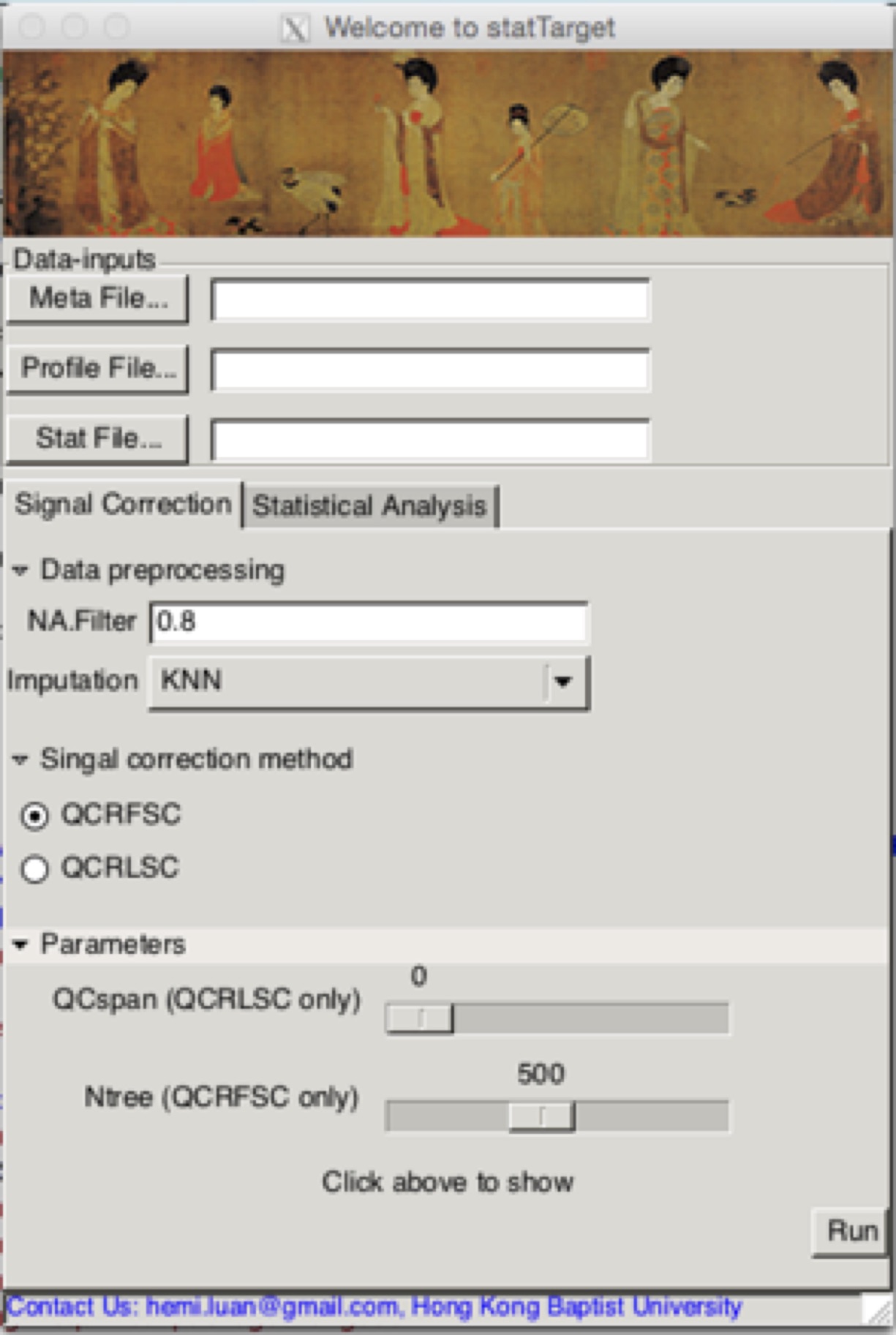
数据校正界面参数解说
Meta File
这里主要是放样本的表型信息,可以参考例子。强烈建议用transX的功能自动输出格式文件,看下文。
表格包含主要这四列。
(1) Class: 分组,QC样本需要标记为NA,即缺失值
(2) Order : 进样序列
(3) Batch: 批次
(4) name: 样品名称,质控样品名称需要包含QC。
*点击,选择你的数据路径
Profile File
组学峰强度数据表
NA.Filter
80%规则过滤缺失值过多的噪音峰
MLmethod
基于机器学习的校正算法(QCRFSC或者QCRLSC)
Ntree
QCRFSC关键参数之一,树数目。
QCspan
QCRLSC关键参数一直,默认0,代表自动优化最优值,防止数据过拟合。
Imputation
数据缺失值或者0值替代。提供四种方法(i.e., nearest neighbor averaging, “KNN”;
minimum values, “min”; Half of minimum values “minHalf”; median values,
“median”. (Default: KNN)
## 如果不想用界面,喜欢用代码得技术宅,看这里

library(statTarget)

datpath <- system.file('extdata',package = 'statTarget')
samPeno <- paste(datpath,'MTBLS79_sampleList.csv', sep='/')
samFile <- paste(datpath,'MTBLS79.csv', sep='/')
shiftCor(samPeno,samFile, Frule = 0.8, MLmethod = "QCRFSC", QCspan = 0,imputeM = "KNN")

See ?shiftCor for off-line help
统计分析界面参数解说 (任意两组比较结果)
Stat File
组学峰强度数据表,包括分组
NA.Filter
80%规则过滤缺失值过多的噪音峰
Imputation
数据缺失值或者0值替代。提供四种方法(i.e., nearest neighbor averaging, “KNN”;
minimum values, “min”; Half of minimum values “minHalf”; median values,
“median”. (Default: KNN)
Normalization
数据标准化方法 (i.e probabilistic quotient
normalization, “PQN”; integral normalization , “SUM”, and “none”).
Glog
Glog转化(正态性)
Scaling Method
数据归一化,用于PCA,PLS-DA分析
Center can be used for specifying the Center scaling.
Pareto can be used for specifying the Pareto scaling.
Auto can be used for specifying the Auto scaling (or unit variance scaling).
Vast can be used for specifying the vast scaling.
Range can be used for specifying the Range scaling. (Default: Pareto)
Permutation times
置换测试次数,越多越好,也会耗费更多的时间。
PCs
第一主成分,第二主成分。得分图显示的横纵坐标。
nvarRF
显示随机森林模型最重要的峰名称。
Labels
得分图是否显示样品名字。
Multiple testing
多重检验,假阳性验证(BH方法)。如果选择TRUE,P值经过BH校正。选择FLASE,则为原始P值。
Volcano FC
火山图倍数阈值
Volcano Pvalue
火山图P值或者假阳性校正P值阈值
## 如果不想用界面,喜欢用代码得技术宅,看这里

library(statTarget)

datpath <- system.file('extdata',package = 'statTarget')
file <- paste(datpath,'data_example.csv', sep='/')
statAnalysis(file,Frule = 0.8, normM = "NONE", imputeM = "KNN", glog = TRUE,scaling = "Pareto")
TransX功能,生成输入表格
transX可以识别当前主流的质谱软件输出的结果,例如XCMS,MZmine2,SKYLINE,进一步生成相应的statTarget需要的表格。
不熟悉XCMS的看官,看这里,http://xcmsonline.scripps.edu ,在线版本分析代谢组学数据。
也可联系本人,愿意提供专业的帮助,QQ 290784996。
## 如果不想用界面,喜欢用代码得技术宅,看这里

library(statTarget)

datpath <- system.file('extdata',package = 'statTarget')
dataXcms <- paste(datpath,'xcmsOutput.tsv', sep='/')
dataSkyline <- paste(datpath,'skylineDemo.csv', sep='/')
transX(dataXcms,'xcms')
transX(dataSkyline,'skyline')

See ?transX for off-line help
结果实例
点击下载实例和报告 Example data and Demo reports
信号校正输出结果 (ShiftCor)
statTarget -- shiftCor
-- After_shiftCor             # The fold for intergrated and corrected data
   -- shift_all_cor.csv         # 校正后的表格,用于下一步统计分析 The corrected data of samples and QCs
   -- shift_QC_cor.csv          # The corrected data of QCs only
   -- shift_sample_cor.csv      # The corrected data of samples only
   -- loplot                    # The fold for quality control images
      -- *.pdf                  # The quality control images for each features

-- Before_shiftCor            # The fold for raw data
   -- shift_QC_raw.csv          # The raw data of QCs
   -- shift_sam_raw.csv         # The raw data of samples

-- RSDresult                  # The fold for variation analysis and quality assessment
   -- RSD_all.csv               # 所有特征峰的RSD值,可用于过滤符合要求的特征峰 The RSD values of each feature
   -- RSDdist_QC_stat.csv       # 所有特征峰的RSD分布 The RSD distribution of QCs in each batch and all batches
   -- RSD distribution.pdf      # The RSD distribution plot in samples and QCs of all batches
   -- RSD variation.pdf         # The RSD variation plot for pre- and post- signal correction
- The status log (Example data):
#############################
# Signal Correction function #
#############################


statTarget: Shift Correction Start... Time: Sun Mar 19 19:43:25 2017

* Step 1: Data File Checking Start..., Time:  Sun Mar 19 19:43:25 2017

 217 Meta Samples vs 218 Profile samples
 The Meta samples list (*NA, missing data from the Profile File)

  [1] "QC1"              "A1"               "A2"               "A3"
  [5] "A4"               "A5"               "QC2"              "A6"
  [9] "A7"               "A8"               "A9"               "A10"
 [13] "QC3"              "A11"              "A12"              "A13"
 [17] "A14"              "A15"              "QC4"              "B16"
 [21] "B17"              "B18"              "B19"              "B20"
 [25] "QC5"              "B21"              "B22"              "B23"
 [29] "B24"              "B25"              "QC6"              "B26"
 [33] "B27"              "B28"              "B29"              "B30"
 [37] "QC7"              "C31"              "C32"              "C33"
 [41] "C34"              "C35"              "QC8"              "C36_120918171155"
 [45] "C37"              "C38"              "C39"              "C40"
 [49] "QC9"              "C41"              "C42"              "C43"
 [53] "C44"              "C45"              "QC10"             "D46"
 [57] "D47"              "D48"              "D49"              "D50"
 [61] "QC11"             "D51"              "D52"              "D53"
 [65] "D54"              "D55"              "QC12"             "D56"
 [69] "D57"              "D58"              "D59"              "D60"
 [73] "QC13"             "E61"              "E62"              "E63"
 [77] "E64"              "E65"              "QC14"             "E66"
 [81] "E67"              "E68"              "E69"              "E70"
 [85] "QC15"             "E71"              "E72"              "E73"
 [89] "E74"              "E75"              "QC16"             "F76"
 [93] "F77"              "F78"              "F79"              "F80"
 [97] "QC17"             "F81"              "F82"              "F83"
[101] "F84"              "F85"              "QC18"             "F86"
[105] "F87"              "F88"              "F89"              "F90"
[109] "QC19"             "QC20"             "a1"               "a2"
[113] "a3"               "a4"               "a5"               "QC21"
[117] "a6"               "a7"               "a8"               "a9"
[121] "a10"              "QC22"             "a11"              "a12"
[125] "a13"              "a14"              "a15"              "QC23"
[129] "b16"              "b18"              "b19"              "b20"
[133] "b21"              "QC24"             "b22"              "b23"
[137] "b24"              "b25"              "b26"              "QC25"
[141] "b27"              "b28"              "b29"              "b30"
[145] "c31"              "QC26"             "c32"              "c33"
[149] "c34"              "c35"              "c36"              "QC27"
[153] "c37"              "c38"              "c39"              "c40"
[157] "c41"              "QC28"             "c42"              "c43"
[161] "c44"              "c45"              "d46"              "QC29"
[165] "d47"              "d48"              "d49"              "d50"
[169] "d51"              "QC30"             "d52"              "d53"
[173] "d54"              "d55"              "d56"              "QC31"
[177] "d57"              "d58"              "d59"              "d60"
[181] "e61"              "QC32"             "e62"              "e63"
[185] "e64"              "e65"              "e66"              "QC33"
[189] "e67"              "e68"              "e69"              "e70"
[193] "e71"              "QC34"             "e72"              "e73"
[197] "e74"              "e75"              "f76"              "QC35"
[201] "f77"              "f78"              "f79"              "f80"
[205] "f81"              "QC36"             "f82"              "f83"
[209] "f84"              "f85"              "f86"              "QC37"
[213] "f87"              "f88"              "f89_120921102721" "f90"
[217] "QC38"

 Warning: The sample size in Profile File is larger than Meta File!

 Meta-information:

  Class No.
1     1  30
2     2  29
3     3  30
4     4  30
5     5  30
6     6  30
7    QC  38
  Batch No.
1     1 109
2     2 108

 Metabolic profile information:

                no.
QC and samples  218
Metabolites    1312

* Step 2: Evaluation of Missing Value...

 The number of missing value before QC based shift correction:  2280
 The number of variables including 80 % of missing value :   3

* Step 3: Imputation start...

 The imputation method was set at 'KNN'
 The number of missing value after imputation:  0
 Imputation Finished!

* Step 4: QC-based Shift Correction Start... Time:  Sun Mar 19 19:43:28 2017

 The MLmethod was set at QCRFC

  |
  |                                                                          |   0%
  |
  |=                                                                         |   1%
  |
  |=                                                                         |   2%
  |
  |==                                                                        |   2%
  |
  |==                                                                        |   3%
   ...
  |========================================================================  |  98%
  |
  |========================================================================= |  99%
  |
  |==========================================================================|  99%
  |
  |==========================================================================| 100%

 High-resolution images output...

  |
  |                                                                          |   0%
  |
  |                                                                          |   1%
  |
  ...
  |========================================================================  |  98%
  |
  |========================================================================= |  99%
  |
  |==========================================================================|  99%
  |
  |==========================================================================| 100%

 Calculation of CV distribution of raw peaks (QC)...

            CV<5%    CV<10%   CV<15%   CV<20%   CV<25%   CV<30%   CV<35%   CV<40%
Batch_1 0.4583652  7.868602 22.84186 36.74561 46.37128 53.32315 60.80978 66.99771
Batch_2 6.5699007 29.870130 49.50344 59.12911 65.62261 70.58824 76.01222 80.67227
Total   0.3819710  6.875477 21.31398 33.68984 44.61421 52.10084 59.12911 65.01146
          CV<45%   CV<50%   CV<55%   CV<60%   CV<65%   CV<70%   CV<75%   CV<80%
Batch_1 72.49809 77.76929 81.05424 84.03361 86.93659 88.54087 89.53400 90.60351
Batch_2 83.34607 86.78380 89.22842 90.98549 92.20779 93.35371 94.27044 94.95798
Total   69.44232 74.17876 78.38044 81.20703 83.11688 85.10313 87.01299 89.99236
          CV<85%   CV<90%   CV<95%  CV<100%
Batch_1 91.59664 92.74255 93.65928 94.88159
Batch_2 95.79832 96.40947 96.71505 97.32620
Total   91.74943 93.43010 94.57601 95.03438

 Calculation of CV distribution of corrected peaks (QC)...

           CV<5%   CV<10%   CV<15%   CV<20%   CV<25%   CV<30%   CV<35%   CV<40%
Batch_1 20.77922 53.93430 70.20626 80.21390 85.71429 89.61039 92.13140 93.58289
Batch_2 33.61345 63.02521 78.38044 86.70741 91.06188 93.88846 94.80519 95.87471
Total   22.76547 54.92743 73.79679 83.11688 88.15890 90.90909 93.04813 94.27044
          CV<45%   CV<50%   CV<55%   CV<60%   CV<65%   CV<70%   CV<75%   CV<80%
Batch_1 94.42322 95.18717 95.79832 96.25668 97.32620 97.86096 98.39572 98.62490
Batch_2 96.25668 97.17341 97.78457 98.16654 98.47212 98.54851 98.54851 98.77769
Total   95.87471 97.02063 97.78457 98.01375 98.39572 98.54851 98.54851 98.62490
          CV<85%   CV<90%   CV<95%  CV<100%
Batch_1 98.85409 98.93048 98.93048 99.23606
Batch_2 99.00688 99.15966 99.15966 99.15966
Total   98.85409 99.00688 99.23606 99.38885

 Correction Finished! Time:  Sun Mar 19 19:44:54 2017
统计分析输出结果 (statAnalysis)
statTarget -- statAnalysis

-- dataSummary                  # The results summaries of basic statistics
-- scaleData_XX                 # The results of scaling procedure
-- DataPretreatment             # Data processed with normalizationor glog transformation procedure.
-- randomForest                 # The results of randomForest analysis and permutation based importance variables.
   -- MultiDimensionalScalingPlot # Multi dimensional scaling plot
   -- VarableImportancePlot       # Varable importance plot

-- PCA_Data_XX                  # Principal Component Analysis with XX scaling
   -- ScorePlot_PC1vsPC2.pdf      # Score plot for 1st component vs 2st component in PCA analysis
   -- LoadingPlot_PC1vsPC2.pdf    # Loading plot for 1st component vs 2st component in PCA analysis

-- PLS_(DA)_XX                  # Partial least squares (-Discriminant Analysis) with XX scaling
   -- ScorePlot_PLS_DA_Pareto     # Score plot for PLS analysis
   -- W.cPlot_PLS_DA_Pareto       # Loading plot for PLS analysis
   -- Permutation_Pareto          # Permutation test plot for PLS-DA analysis (for two groups only)
   -- PLS_DA_SPlot_Pareto         # Splot plot for PLS analysis

-- Univariate
   ----- BoxPlot
   ----- Fold_Changes             # A ratio of feature between control and case
   ----- Mann-Whitney_Tests       # For non-normally distributed variables
   ----- oddratio                 # Odd ratio
   ----- Pvalues                  # 值得推荐,五颗星!!!,P值得结果,综合考虑数据正态性,如果数据正态分布,则是WelchTest结果,非正态分布,则是Mann-Whitney_Tests结果。Integration of pvalues or BH-adjusted pvalues for normal data (Welch test) and abnormal data (Mann Whitney Tests)
   ----- ROC                      # Receiver operating characteristic curve
   ----- Shapiro_Tests            # Normality tests
   ----- Significant_Variables    # The features with P-value < 0.05
   ----- Volcano_Plots            # P-value and fold Change scatter plot
   ----- WelchTest                # For normally distributed variables

- The status log (Example data):
#################################
# Statistical Analysis function #
#################################


statTarget: statistical analysis start... Time:  Tue May  9 19:50:53 2017

* Step 1: Evaluation of missing value...

 The number of missing value in Data Profile:  0
 The number of variables including 80 % of missing value :   0

* Step 2: Summary statistics start... Time:  Tue May  9 19:50:53 2017

* Step 3: Missing value imputation start... Time:  Tue May  9 19:50:53 2017

 Imputation method was set at KNN
 The number of NA value after imputation: 0
 Imputation Finished!
* Step 4: Normalization start... Time:  Tue May  9 19:50:59 2017

 Normalization method was set at NONE

* Step 5: Glog PCA-PLSDA start... Time:  Tue May  9 19:51:01 2017

 Scaling method was set at Center

 PCA Model Summary
 59 samples x 1309 variables
 Variance Explained of PCA Model:

                            PC1      PC2      PC3      PC4     PC5
Standard deviation     4.651009 4.452616 3.963728 3.180499 2.66858
Proportion of Variance 0.143390 0.131420 0.104140 0.067050 0.04720
Cumulative Proportion  0.143390 0.274810 0.378950 0.446000 0.49320

 The following observations are calculated as outliers: [1] "A13" "A14"

 PLS(-DA) Two Component Model Summary
 59 samples x 1309 variables
 Fit method: oscorespls
 Number of components considered: 2
 Cross-validated using 10 random segments.

 Cumulative Proportion of Variance Explained: R2X(cum) = 19.34905%
 Cumulative Proportion of Response(s):

                Y1        Y2
R2Y(cum) 0.9391357 0.9391357
Q2Y(cum) 0.8175050 0.8175050

 Permutation of PLSDA Model START...!

  |
  |                                                                               |   0%
  ...
  |===============================================================================|  99%
  |
  |===============================================================================| 100%

* Step 6: Glog Random Forest start... Time:  Tue May  9 19:52:03 2017


  |
  |                                                                               |   0%
  |
  ...
  |============================================================================== |  98%
  |
  |============================================================================== |  99%
  |
  |===============================================================================|  99%
  |
  |===============================================================================| 100%

 Random Forest Model
 Type:  classification
 ntree: 500
 mtry:  36
 OOB estimate of error rate: 0 %

 Permutation-based Gini importance measures
 The number of permutations:  500
 Selected 50 variables with top importance

          1          2          3          4          5          6          7
giniImp   "M302T751" "M301T716" "M304T768" "M113T110" "M279T716" "M305T103" "M117T584"
pvalueImp "M301T716" "M302T751" "M113T110" "M239T109" "M304T768" "M280T750" "M279T716"
          8          9          10         11         12         13         14
giniImp   "M280T750" "M239T109" "M265T768" "M311T103" "M379T103" "M243T104" "M281T750"
pvalueImp "M191T105" "M302T716" "M265T768" "M305T103" "M281T750" "M243T104" "M117T584"
          15         16         17         18         19         20         21
giniImp   "M191T105" "M457T107" "M249T108" "M315T110" "M267T106" "M302T716" "M161T728"
pvalueImp "M311T103" "M379T103" "M249T108" "M283T767" "M267T106" "M305T768" "M315T110"
          22         23         24         25         26         27         28
giniImp   "M283T767" "M305T768" "M348T761" "M297T705" "M355T120" "M259T104" "M263T750"
pvalueImp "M348T761" "M355T120" "M457T107" "M297T705" "M353T761" "M243T754" "M263T750"
          29         30         31         32         33         34         35
giniImp   "M88T588"  "M325T774" "M290T728" "M353T761" "M373T102" "M243T754" "M241T109"
pvalueImp "M241T109" "M107T105" "M259T104" "M325T774" "M290T728" "M161T728" "M262T112"
          36         37         38         39         40           41         42
giniImp   "M338T716" "M262T112" "M107T105" "M381T802" "M165T109_1" "M361T748" "M295T728"
pvalueImp "M381T802" "M338T716" "M88T588"  "M373T102" "M165T109_1" "M261T113" "M295T728"
          43         44         45         46         47         48         49
giniImp   "M239T116" "M261T113" "M205T716" "M761T800" "M269T771" "M283T112" "M257T762"
pvalueImp "M361T748" "M239T116" "M263T115" "M360T748" "M123T105" "M175T104" "M269T771"
          50
giniImp   "M123T105"
pvalueImp "M257T762"

* Step 7: Univariate Test Start...! Time:  Tue May  9 20:01:26 2017

 P-value Calculating...
 P-value was adjusted using Benjamini-Hochberg Method

 Odd.Ratio Calculating...

 ROC Calculating...

  |
  |                                                                               |   0%
  |
  |                                                                               |   1%
  |
  |=============================================================================  |  98%
  |
  |============================================================================== |  98%
  |
  |============================================================================== |  99%
  |
  |===============================================================================|  99%
  |
  |===============================================================================| 100%

 Volcano Plot and Box Plot Output...

 Statistical Analysis Finished! Time:  Tue May  9 20:03:50 2017
References
Luan H.,(2018) statTarget: A streamlined tool for signal drift correction and interpretations of quantitative mass spectrometry-based omics data. Analytica Chimica Acta. dio: https://doi.org/10.1016/j.aca.2018.08.002
Luan H.,(2018) Quality control-based signal drift correction and interpretations of metabolomics/proteomics data using random forest regression. bioRxiv 253583; doi: https://doi.org/10.1101/253583
Luan H., LC-MS-Based Urinary Metabolite Signatures in Idiopathic
Parkinson’s Disease. J Proteome Res., 2015, 14,467.
Luan H., Non-targeted metabolomics and lipidomics LC-MS data
from maternal plasma of 180 healthy pregnant women. GigaScience 2015 4:16